In 2012-2013 I travelled to several remote First Nations communities around British Columbia to do hands-on mathematical activities with elementary school kids and teachers. Math Catcher, which provided the free math presentations, has also born several mathematical stories about a young boy, named Small Number, that have been translated into Aboriginal languages from across Canada. I have embedded all of Small Number’s stories and translations here (updated 31 August 2016) for your ears to enjoy the sound of these languages.

Click here to support this program directly by giving to Simon Fraser University.

Small Number Counts to 100

Written by Veselin Jungic & Mark MacLean Illustrated by Simon Roy.

Small Number and the Old Canoe

Written by Veselin Jungic & Mark MacLean Illustrated by Simon Roy

Small Number and the Basketball Tournament

Written by Veselin Jungic, SFU, and Mark MacLean, UBC Illustrated by Jean-Paul Csuka, Canada

Small Number and the Big Tree

Written by Veselin Jungic and Mark MacLean Illustrated by Simon Roy and Jess Pollard

Small Number and the Skateboard Park

Written by Veselin Jungic & Mark MacLean Illustrated by Simon Roy

Small Number and the Salmon Harvest

Written by Veselin Jungic & Mark MacLean Illustrated by Simon Roy & Jess Pollard

Small Number and the Old Totem Pole

Written by Veselin Jungic and Mark MacLean Illustrated by Bethani L’Heureux

I am unfamiliar with these (and all) Aboriginal languages, so please let me know if I have made any errors in this blog post, and especially if the special characters are not rendering correctly.

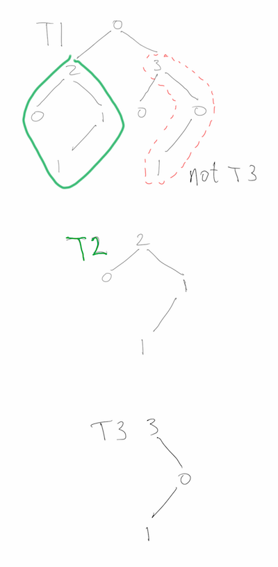
“Cracking the Coding Interview 6e” question 4.10: T1 and T2 are binary trees with m and n nodes, respectively. Test whether T1 contains T2 as a subtree. Here is my solution, which performs much better than the book’s solution.

The problem asks, more specifically, if there is a node in T1 such that the subtree rooted there has exactly the same structure as T2, as well as the same values at each node. Spoilers follow the image below, so if you are looking for hints, proceed carefully.

Test subtree containment

CCtI6e discusses two solutions, the first one makes the observation that a tree is uniquely identified by its pre-order traversal if you include special identifiers for null child-nodes, so the tree containment problem is reduced to a substring problem: does toString(T1) contain toString(T2)? CCTI6e blurs the solution by using a library call to solve the substring problem (it is not trivial to do it efficiently), but they do claim that this solution runs in O(m+n) time and O(m+n) space. It’s a valid answer, but I want something better.

The second solution tries to improve on the O(m+n) space of the first solution. The naïve way would be to do a depth-first search comparison of T2 and the subtree rooted at each node of T1, resulting in an O(log(m) + log(n)) space algorithm that uses O(min(m*log(m),m*n)) time. CCtI6e suggests using the values of the root of the T1-subtree and the root of T2 to decide whether or not to perform the search, but this ultimately makes no difference at all. First, if the values are different, then the search would abort immediately, and second, the nodes of T1 and T2 could have all the same data, say 0. Below is a drawing of a bad case, where most of T2 occurs at many nodes of T1, but T1 does not contain T2.

A bad case for recursive subtree testing

I was surprised to see such naïve solution to this problem, as CCtI6e has been very good so far. The recursive solution can be improved upon considerably by using a better heuristic for whether or not to search/compare T2 with the subtree at a given node of T1.

Hash the structure and data of a binary tree

We want to hash each node so that if the hashes of two trees match, there is a high probability that their subtrees match. As a proof of concept, I adapted Knuth’s multiplicative method to work on binary trees with integer values. The idea is to re-hash the hash values of the left and right children, as well as the height and value of the current node, using distinct 32-bit primes for each part, and then add the four multiplicative hash values. I’ve read that hashing is part guess-work and part theory, and there you have it.

uint32_t hash(uint64_t left,
              uint64_t right,
              uint64_t value,
              uint64_t height){
  return ((left&(0xFFFFFFFF))*2654435761 +
          (right&(0xFFFFFFFF))*2654435741 +
          (value&(0xFFFFFFFF))*2654435723 +
          (height&(0xFFFFFFFF))*2654435713);
}

uint32_t dfs_hash(node *t){
  if(!t) return 0;
  return hash(dfs_hash(t->left),dfs_hash(t->right),t->value,t->height);
}

My hash function seems to work quite well for randomly generated trees, but it is not thoroughly tested or anything. I’d like to eventually adapt a more sophisticated function, perhaps from Eternally Confuzzled.

Using the tree-hashes

My algorithm works as follows:

• pre-compute the hash of T2.
• Do a depth-first search of T1 where at each node:
  • if one of child nodes of the current node contains T2, return True. Otherwise, record the hashes of the child nodes.
  • hash the current node in O(1) time
  • if the hash of the current node matches the hash of T2:
    • do a depth-first search that compares T2 to the subtree rooted at the current node
    • if T2 is identical to the subtree rooted at the current node, then return True
  • return the hash of the current node.

Note that I do not cache hash values. The idea in this exercise is not to use unnecessary space, beyond the O(log(m)+log(n)) space necessarily used by depth-first searches. Caching hash values would not only use O(n+m) additional space, but keeping the hash values up to date in a non-static binary tree requires modifying the binary tree implementation.

The above pseudo-code is implemented below, and the complete source-code is at the end of this blog post.

typedef struct node{
  int value,height;
  struct node *left;
  struct node *right;
}node;

node *rec_contains_subtree(node *t1, node *t2, uint32_t *t1ChildHash, uint32_t t2hash){
  uint32_t leftChildHash,rightChildHash;
  node *res;
  *t1ChildHash=0;
  if(!t1)
    return NULL;
  if((res=rec_contains_subtree(t1->left,t2,&leftChildHash, t2hash))||
     (res=rec_contains_subtree(t1->right,t2,&rightChildHash,t2hash)))
    return res;
  count_nodes_hashed++;
  *t1ChildHash=hash(leftChildHash,rightChildHash,t1->value,t1->height);
  if(*t1ChildHash==t2hash){
    count_dfs_compare++;
    if(dfs_compare_trees(t1,t2))
      return t1;
  }
  return NULL;
}

node *contains_subtree(node *t1, node *t2){
  //hash t2
  uint32_t t2hash = dfs_hash(t2);
  uint32_t t1ChildHash;
  if(!t2)
    exit(-1);
  return rec_contains_subtree(t1,t2,&t1ChildHash,t2hash);
}

Below is the other depth-first search, that compares T2 with a subtree of T1. Notice that the CCtI6e solution is implicit in the last conditional.

int dfs_compare_trees(node *t1, node *t2){
  if(!t1 && !t2)
    return 1;
  if(!t1 && t2)
    return 0;
  if(t1 && !t2)
    return 0;
  if(t1->value!= t2->value)
    return 0;
  return dfs_compare_trees(t1->left,t2->left) &&
    dfs_compare_trees(t1->right,t2->right);
}

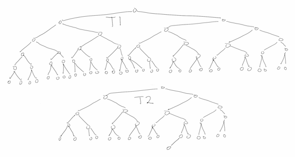
Testing on some large inputs

I did some tests on randomly generated trees. This is by no means a robust test, especially as regards hash collisions. I’ll paste some output and then explain it.

Below, I insert 10,000,000 nodes into T1 and 100 nodes into T1, by descending the trees on randomly selected branches and inserting at the first empty node. All data values are 0s. Since the result is that T1 doesn’t contain T2, then all 10,000,000 nodes of T1 are searched, but notice that the hashing saves me from doing any node-by-node comparisons with T2.

1e-05 seconds to allocate trees
10.3298 seconds to create t1
2e-05 seconds to create t2
t1 has 10000000 nodes
t2 has 100 nodes
0.928297 seconds to check if t1 contains t2
t1 does not contain t2
Did dfs_compare_trees 0 times
Hashed 10000000 nodes of t1

With the same tree T1 as above, I regenerated T2 100 times and repeated the same test as above. Again, the node-by-node comparison, dfs compares, was done 0 times (per search).

Test containment in t1 of randomly generated trees t2
Nodes: t1 10000000 t2 100; Trials: 100
All nodes hold value=0
Average per search:
	time 0.944213;
	dfs compares 0;
	prop. nodes hashed 1;
	containment 0

I repeated the previous experiment, below, with smaller trees T2, on 20 nodes. Now we see that 6/100 of these T2s are contained in T1, but dfs_compares is done 10 times more often than we find something. It shows that the hashing is giving quite a few false positives for small T2! More testing needed.

Test containment in t1 of randomly generated trees t2
Nodes: t1 10000000 t2 20; Trials: 100
All nodes hold value=0
Average per search:
	time 0.96471;
	dfs compares 0.58;
	prop. nodes hashed 0.964319;
	containment 0.06

In order to test containment of larger trees T2, I simply used subtrees of T1, selected (pseudo) uniformly at random. Since my search does not consider the values of the references to the nodes, it is unaware that T1 and T2 share locations in memory. Below we see that very few nodes of T1 are hashed, and that a hash collision is experienced in about 12% of the searches, since 1.12=dfs_compares/containment.

Test containment in t1 of randomly selected subtrees of t1
Nodes: t1 10000000 t2 (unknown); Trials: 100
All nodes hold value=0
Average per search:
	time 0.0682518;
	dfs compares 1.12;
	prop. nodes hashed 0.0711984;
	containment 1

The running time is difficult to compute (and maybe impossible to prove), because of the way it depends on the hash function. Informally, we can state an expected time of O(m+(1+c)n), where c is the number of hash collisions. If c is small enough, this becomes O(m). This is much better than CCtI6e’s time of O(m+kn), where k is the number of nodes of T1 that have the same value as the root of T2, since, in our 0-value trees, that could easily amount to O(m*log(m)); the cost of doing a full depth-first search of T1 at every node.

The code, which is a bit rough and quick, is available as a gist:

I saw a nice question on leetcode today, apparently asked recently at a Google on-site interview.

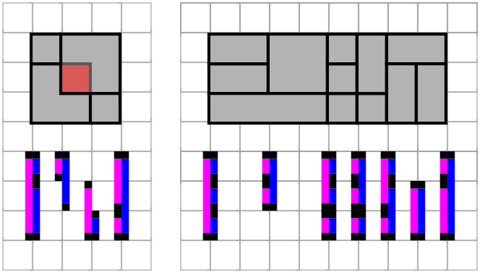
Given N rectangles with integer coordinates, check whether they are an exact cover of a rectangular region

If you don’t know already, Google’s on-site interview process involves 5 independent interviews in one day. In each one a Google Software Engineer poses a problem that should be solved in 45 min to 1 hr. The interviewee can code on a white board or in Google Docs (check with your recruiter for details) in a language of their choice, but not pseudo-code.

By itself, the question is not all that intimidating, but the time-limit can make it quite challenging. That’s why I’m practising!

As usual, there is a fairly straightforward “brute force” solution, and some better solutions. I’ll give hints and solutions immediately after the jump so avoid spoilers by not looking past the example inputs yet.

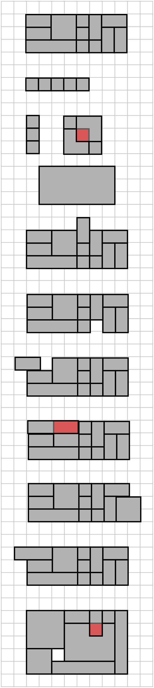
Example inputs

Hint 1

Try to find a brute-force solution by looking at the total area of the rectangles.

Hint 2

After computing the area, can you avoid comparing every pair of rectangles?

Hint 3

The problem can be solved in O(N log N), both with and without computing areas.

Hint 4

What needs to occur at every left-hand segment of an input rectangle that is interior to the smallest rectangle that bounds the input rectangles? At every right-hand segment? At the vertical segments not interior?

Solutions from area

One solution is to compute the area of the smallest bounding rectangle, and the combined areas of the N input rectangles. The input data is unsorted, so you need to do an O(N) scan of the input to find the minimum and maximum points, both vertically and horizontally (up to 4 points). If the areas differ, output False, and if they are the same, you need to check that no pair of input rectangles intersect. To see why, look at the input below.

Area problem input

Testing whether a pair of rectangles intersect is a simple, O(1) calculation (though I would understand if you failed to get it onto the whiteboard in 5 minutes under pressure), so we know we can finish in O(N^2) time by comparing (N choose 2) pairs of input rectangles.

Some light reading suggests that the intersections can be tested in O(N log N) time in some cases, but the solutions seem far from simple. I didn’t look at this very deeply, but for further reading:

R-trees on StackOverflow
R-trees on Wikipedia
Another answer on StackOverflow
The Princeton lecture cited in the above StackOverflow answer

I’ll now present a solution that does not require any 2D geometric tests.

My Solution

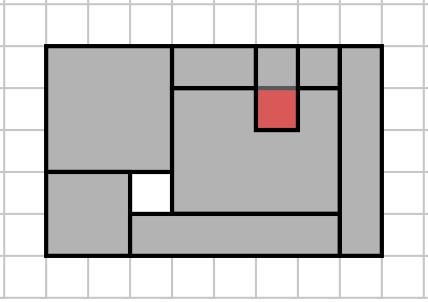
Imagine, first, that the (smallest) rectangle bounding the inputs is a cylinder, so that its leftmost edge coincides with its rightmost edge. Now we can state the ‘algorithm’ in one sentence:

If (P) every point interior to a right-hand edge of an input rectangle is unique, and it coincides with a point of a left-hand edge of an input rectangle, and vise versa, then we (Q) output True, and otherwise we output False.

Take a moment to let that sink in. We are claiming that P if and only if Q. Let us make clear here that when we say rectangles intersect, we mean that their interiors intersect. The explanation is a bit dense, but hopefully you’ll come to the same conclusions by making some drawings.

isBigRect uses the interfaces of vertical segments

If P is false, then one of two things can happen. If points interior to the right-hand edges of two distinct rectangles coincide, then the rectangles intersect. Otherwise, without loss of generality, we may assume there is there is some point p on a left-hand edge of an input rectangle, call it A, that does not coincide with a point on a right-hand edge of an input rectangle. Thus, p is interior to a small open disc that both contains points interior to A and points exterior to A. The same disc is either entirely inside a rectangle distinct from A, which will necessarily intersect with A, or it contains points exterior to all rectangles distinct from A, and thus contains a hole in the bounding cylinder. Thus we output False, so Q is false.

If Q is false, on the other hand, then either two distinct rectangles intersect, or a point in the bounding cylinder falls outside of all input rectangles. If rectangles intersect and they have intersecting vertical segments, then P is false, so we may assume that is not the case. But then, the vertical segment of one rectangle must be interior to another rectangle, which again falsifies P. Finally, if a point falls outside of all rectangles, then there are vertical segments to its left and right that falsify P.

Thus, we have shown that P is a necessary and sufficient condition for the N rectangles to be an exact cover of a rectangle, q.e.d.

Now we need to code the solution. The short of it is, we sort a copy of the input rectangles by left-edge x-coordinates, and we sort another copy by right-edge x-coordinates. The first left edge and last right edge are special cases, but are easily dealt with. We then process the vertical segments in the sorted lists, at each x-coordinate, and simply compare the lists.

The bottleneck in time-complexity is in sorting the inputs, plus we need O(N) space to make left-edge-sorted and right-edge-sorted copies of the inputs.

I am assuming that an input rectangle is given as a bottom-left point and a top-right point; for example, a unit square is [[1,1],[2,2]].

A final word of warning before you delve into my Python code. I am primarily a C-programmer leveraging some features of Python, so my code is not very “Pythonic”. Suggestions, improvements, and more test cases welcome.

def isBigRect(rectangles):
    if rectangles==[]:
        return True
    L=processBoundaries(rectangles,leftOrRight='left')
    R=processBoundaries(rectangles,leftOrRight='right')
    if L==False or R==False or not len(L)==len(R):
        return False
    L[-1][0]=R[-1][0]
    R[0][0]=L[0][0]
    if not L==R:
        return False
    else:
        return True

def processBoundaries(B,leftOrRight='left'):
    x0orx1=0
    if leftOrRight=='right':
        x0orx1=1
        res=[[]]
    elif leftOrRight=='left':
        x0orx1=0
        res=[]
    else:
        print 'process boundaries input error'
        return False
    B=[ [x[x0orx1][0],[x[0][1],x[1][1]]] for x in B]
    B.sort(cmp=lambda x,y: x[0]-y[0])
    i=0
    while i<len(B):
        x=B[i][0]
        res.append( [x,[]] )
        while i<len(B) and B[i][0]==x:
            res[-1][1].append(B[i][1])
            i=i+1
        res[-1][1]=mergeSpecialIntervals(res[-1][1])
        if res[-1][1]==False:
            return False
    if leftOrRight=='right':
        res[0]=['first',res[-1][1]]
    else:
        res.append(['last',res[0][1]])
    return res

def mergeSpecialIntervals(L):
    if L==[]:
        return False
    if len(L)==1:
        return L
    L.sort(cmp=lambda x,y: x[0]-y[0])
    res=[L[0]]
    for i in range(len(L)-1):
        if L[i][1]>L[i+1][0]:
            return False
        elif L[i][1]==L[i+1][0]:
            res[-1][1]=L[i+1][1]
            i=i+2
        else:
            res.append(L[i])
            i=i+1
    if i == len(L)-1:
        res.append(L[i])
    return res


A=[[[[0,0],[4,1]],
    [[7,0],[8,2]],
    [[6,2],[8,3]],
    [[5,1],[6,3]],
    [[4,0],[5,1]],
    [[6,0],[7,2]],
    [[4,2],[5,3]],
    [[2,1],[4,3]],
    [[0,1],[2,2]],
    [[0,2],[2,3]],
    [[4,1],[5,2]],
    [[5,0],[6,1]]],

   #shuffled the above a little
   [[[0,0],[4,1]],
    [[7,0],[8,2]],
    [[5,1],[6,3]],
    [[6,0],[7,2]],
    [[4,0],[5,1]],
    [[4,2],[5,3]],
    [[2,1],[4,3]],
    [[0,2],[2,3]],
    [[0,1],[2,2]],
    [[6,2],[8,3]],
    [[5,0],[6,1]],
    [[4,1],[5,2]]],

   [[[0,0],[4,1]]],

   [],

   #vertical stack
   [[[0,0],[1,1]],
	[[0,1],[1,2]],
	[[0,2],[1,3]],
	[[0,3],[1,4]],],
   
   #horizontal stack
   [[[0,0],[1,1]],
	[[1,0],[2,1]],
    [[2,0],[3,1]],
    [[3,0],[4,1]],],

   ]

print 'should be True'
for a in A:
    print isBigRect(a)


B=[
    #missing a square
    [[[0,0],[4,1]],
     [[7,0],[8,2]],
     [[6,2],[8,3]],
     [[5,1],[6,3]],
     [[6,0],[7,2]],
     [[4,2],[5,3]],
     [[2,1],[4,3]],
     [[0,1],[2,2]],
     [[0,2],[2,3]],
     [[4,1],[5,2]],
     [[5,0],[6,1]]],
    
    #exceeds top boundary
    [[[0,0],[4,1]],
     [[7,0],[8,2]],
     [[5,1],[6,4]],
     [[6,0],[7,2]],
     [[4,0],[5,1]],
     [[4,2],[5,3]],
     [[2,1],[4,3]],
     [[0,2],[2,3]],
     [[0,1],[2,2]],
     [[6,2],[8,3]],
     [[5,0],[6,1]],
     [[4,1],[5,2]]],
    
    #two overlapping rectangles
    [[[0,0],[4,1]],
     [[0,0],[4,1]]],
    
    #exceeds right boundary
    [[[0,0],[4,1]],
     [[7,0],[8,3]],
     [[5,1],[6,3]],
     [[6,0],[7,2]],
     [[4,0],[5,1]],
     [[4,2],[5,3]],
     [[2,1],[4,3]],
     [[0,2],[2,3]],
     [[0,1],[2,2]],
     [[6,2],[8,3]],
     [[5,0],[6,1]],
     [[4,1],[5,2]]],

    # has an intersecting pair
    [[[0,0],[5,1]],
     [[7,0],[8,2]],
     [[5,1],[6,3]],
     [[6,0],[7,2]],
     [[4,0],[5,1]],
     [[4,2],[5,3]],
     [[2,1],[4,3]],
     [[0,2],[2,3]],
     [[0,1],[2,2]],
     [[6,2],[8,3]],
     [[5,0],[6,1]],
     [[4,1],[5,2]]],
    
    #skips column 4
    [[[0,0],[4,1]],
     [[7,0],[8,2]],
     [[5,1],[6,3]],
     [[6,0],[7,2]],
     [[2,1],[4,3]],
     [[0,2],[2,3]],
     [[0,1],[2,2]],
     [[6,2],[8,3]],
     [[5,0],[6,1]],],


    #exceed left boundary
    [[[0,0],[4,1]],
     [[7,0],[8,2]],
     [[5,1],[6,3]],
     [[6,0],[7,2]],
     [[4,0],[5,1]],
     [[4,2],[5,3]],
     [[2,1],[4,3]],
     [[-1,2],[2,3]],
     [[0,1],[2,2]],
     [[6,2],[8,3]],
     [[5,0],[6,1]],
     [[4,1],[5,2]]],


   #horizontal stack with overlapping left boundaries at x=1
    [[[0,0],[1,1]],
     [[1,0],[2,1]],
     [[1,0],[3,1]],
     [[3,0],[4,1]],],
]

print 'should be False'
for b in B:
    print isBigRect(b)

Bonus: what if the input rectangles can be moved?

If you are a mathematician you might be inclined to view a rectangle as simply a width and height, with no fixed location in the plane. This is exactly what Tony Huynh, self-described Mathematical Vagabond (and matroid theorist by trade), pointed out to me, so I asked him if the alternate interpretation of the problem is NP-hard?

The new problem:

Given N rectangles with integer dimensions, check whether they can be translated and rotated to exactly cover a rectangular region.

Indeed the answer is yes, and Tony came back to me a few minutes later with this very nice reduction:

Consider the following input of rectangles, where a rectangle is given by a pair (height, width): (1,a1), (1,a2), …, (1,aN) and (S,S) where S is half the sum of all the ai. If you can solve the rectangle partitioning problem for this instance, then you can find a subset of a1, …, aN whose sum is exactly half the total sum (which is NP-hard).

Suppose you have two unsigned 16-bit integers,
X=0000 0000 0111 1111 1000 1010 0010 0100
and
Y=0000 0000 0000 0000 0011 0000 1010 1111.
How can you tell if Y is more than half as long as X? I came across this because I wanted some code to branch on whether or not Y was a lot bigger or smaller than the square root of a large positive integer X (behaviour when Y was around the square root was arbitrary). The square root of X has half as many bits as X does, and I figured that I could get the lengths of these numbers super fast to make a fairly coarse comparison.

I was right about that, but the efficiency of the answer depends on the CPU the code is running on. Even so, the portable answers should be quite fast, and they are interesting, so let’s look at them.

As usual, I did some research on the internet for this, and the bit twiddling I did is from Stackoverflow and Haacker’s Delight (it’s a book, of course, but I linked to some snippets on their website).

I wrote some code that explains the steps of a smearing function and a population count. In fact, that’s the spoiler: I will smear the bits of X to the right, and then count the population of 1-bits.

//smear
x = x | x>>1;
x = x | x>>2;
x = x | x>>4;
x = x | x>>8;
x = x | x>>16;

//population count
x = ( x & 0x55555555 ) + ( (x >> 1 ) & 0x55555555 );
x = ( x & 0x33333333 ) + ( (x >> 2 ) & 0x33333333 );
x = ( x & 0x0F0F0F0F ) + ( (x >> 4 ) & 0x0F0F0F0F );
x = ( x & 0x00FF00FF ) + ( (x >> 8 ) & 0x00FF00FF );
x = ( x & 0x0000FFFF ) + ( (x >> 16) & 0x0000FFFF );

The idea behind the population count is to divide and conquer. For example with 01 11, I first count the 1-bits in 01: there is 1 1-bit on the right, and there are 0 1-bits on the left, so I record that as 01 (in place). Similarly, 11 becomes 10, so the updated bit-string is 01 10, and now I will add the numbers in buckets of size 2, and replace the pair of them with the result; 1+2=3, so the bit string becomes 0011, and we are done. The original bit-string is replaced with the population count.

There are faster ways to do the pop count given in Hacker’s Delight, but this one is easier to explain, and seems to be the basis for most of the others. You can get my code as a Gist here..

X=0000 0000 0111 1111 1000 1010 0010 0100
Set every bit that is 1 place to the right of a 1
0000 0000 0111 1111 1100 1111 0011 0110
Set every bit that is 2 places to the right of a 1
0000 0000 0111 1111 1111 1111 1111 1111
Set every bit that is 4 places to the right of a 1
0000 0000 0111 1111 1111 1111 1111 1111
Set every bit that is 8 places to the right of a 1
0000 0000 0111 1111 1111 1111 1111 1111
Set every bit that is 16 places to the right of a 1
0000 0000 0111 1111 1111 1111 1111 1111
Accumulate pop counts of bit buckets size 2
0000 0000 0110 1010 1010 1010 1010 1010
Accumulate pop counts of bit buckets size 4
0000 0000 0011 0100 0100 0100 0100 0100
Accumulate pop counts of bit buckets size 8
0000 0000 0000 0111 0000 1000 0000 1000
Accumulate pop counts of bit buckets size 16
0000 0000 0000 0111 0000 0000 0001 0000
Accumulate pop counts of bit buckets size 32
0000 0000 0000 0000 0000 0000 0001 0111

The length of 8358436 is 23 bits

Y=0000 0000 0000 0000 0011 0000 1010 1111
Set every bit that is 1 place to the right of a 1
0000 0000 0000 0000 0011 1000 1111 1111
Set every bit that is 2 places to the right of a 1
0000 0000 0000 0000 0011 1110 1111 1111
Set every bit that is 4 places to the right of a 1
0000 0000 0000 0000 0011 1111 1111 1111
Set every bit that is 8 places to the right of a 1
0000 0000 0000 0000 0011 1111 1111 1111
Set every bit that is 16 places to the right of a 1
0000 0000 0000 0000 0011 1111 1111 1111
Accumulate pop counts of bit buckets size 2
0000 0000 0000 0000 0010 1010 1010 1010
Accumulate pop counts of bit buckets size 4
0000 0000 0000 0000 0010 0100 0100 0100
Accumulate pop counts of bit buckets size 8
0000 0000 0000 0000 0000 0110 0000 1000
Accumulate pop counts of bit buckets size 16
0000 0000 0000 0000 0000 0000 0000 1110
Accumulate pop counts of bit buckets size 32
0000 0000 0000 0000 0000 0000 0000 1110

The length of 12463 is 14 bits

So now I know that 12463 is significantly larger than the square root of 8358436, without taking square roots, or casting to floats, or dividing or multiplying.

It needs to be said that there are built-in functions that get the number of leading or trailing 0s. They are __builtin_clz() and __builtin_ctz() (i.e., clz = count leading zeros), and I read that most modern CPUs will do this computation in 1 instruction. So, alternatively, the length of uint32_t x is

32-__builtin_clz(x);

In doing a simple programming exercise while preparing for a job interview, I decided to sort the input. I wrote a solution for the exercise in 10 minutes, and then spent the next two days implementing “all of the basic sorting algorithms”. When I finally had bubble sort, insertion sort, selection sort, quicksort (with various types of pivots), shell sort, heap sort, radix sort (base 16, no mod operator or division), merge sort, and bogo sort implemented, I wrote some code to test and time the different sorts with various inputs.

Benchmark inputs

“What is the best sorting algorithm?” I have seen this question a dozen times, and the best answer is, invariably: it depends what you are sorting. Not only does it depend on the length of the input array, it also depends on how sorted you expect it to be in the first place, and whether or not the array values are bounded. For example, insertion sort is worst case quadratic, but it’s still extremely fast for long arrays that are already nearly sorted. It’s also faster than it’s asymptotically better counterparts on very short input arrays. For arrays with only small values, radix sort (with counting sort as a subroutine) provides near-linear sort-time. What if you have many small values and a few large ones?

Choosing the best sorting algorithm is as much about knowing what you sorting as it is about the relative performance of the algorithms.

What, then, are some good benchmarks? A lot of data “in the wild” is already sorted, either mostly or completely, so (mostly) pre-sorted inputs are a must. The sort order of the data might also be opposite the sort order of the sorting algorithm, and in many cases this is the difference between best and worst case performance. We already have five benchmark properties to try:

• Unsorted
• Sorted
• Mostly sorted
• Reverse sorted
• Reverse mostly sorted

We might have a large amount of data that is keyed on just a few unique values, or that is keyed only on small values (think radix or counting sort). Perhaps we have a lot of small keys and a few large keys. Here are a few properties that can be combined with the above:

• Few unique keys
• Many unique keys
• Only small keys
• Mostly small keys

And finally, we may be sorting very short arrays frequently:

• One long array
• Many short arrays

My sorting algorithms are all offline and they work only in memory, so measuring CPU cycles should give a realistic comparison.

Experiment setup

I generated a table for each sorting algorithm, with key-related properties and array-size in the rows, and pre-sorting properties in the columns. The details of the properties are as follows:

• Few unique keys:
  Values in range [0,49] are generated at random (see notes on randomness below), and then multiplied by 100,000,000.
• Many unique keys:
  Values in range [0, 1000 000 000] are generated at random.
• Only small keys:
  Values in range [0,49] are generated at random.
• Mostly small keys:
  I did not run this experiment.

The presorting combinations are the ones mentioned in Benchmark inputs, above, and the details of mostly sorted are as follows: sort the array and divide into consecutive bins of size 10. Shuffle the elements in each bin, and reverse if needed.

For each ( key, pre-sorting )-pair I computed the cumulative time to do 1000 small arrays, and the mean times to do 100 medium arrays and 10 large arrays. I had to adjust the size of the large array for some of the slow (in the worst case) algorithms. Both input size, n, and trials, t, are given in the tables.

Random ints are obtained with random() (which is more uniform than rand()), using a technique I learnt on Stack Exchange. I will make a separate post about this later.

int rand_uniform(int min, int max){
  //computing random number in range [0,range)
  //using unsigned long to ensure no overflow of RAND_MAX+1
  unsigned long range=max-min+1;
  if(range<1){
    fprintf(stderr,"Invalid range to random number generator\n");
    exit(-1);
  }
  unsigned long bin_size=((unsigned long)RAND_MAX+1)/range;
  unsigned long limit=range*bin_size;
  unsigned long x;
  //this will execute an expected < 2 times
  do x=random(); while(x>=limit);
  return x/bin_size+min;
}

Results

I benchmarked 9 sorting algorithms in 3 groups, according to the largest inputs they could handle in the worst cases. The choices of input lengths are somewhat ad hoc, but I tried to maintain some comparability between groups by making the medium length inputs of the first and second groups the same as the longest inputs of the next group, respectively, as well as making the smallest inputs all of length 100.

The first group comprises the worst case O(n log(n) ) algorithms, as well as radix sort and shell sort:

• mergesort
• radix sort
• heap sort
• shell sort

The second group is all quicksort, which has a worst case of O( n^2 ):

• quicksort with random pivot
• quicksort with sampled pivot (median of 11 random elements)
• quicksort with A[0] pivot

And finally, the last group contains the quadratic sorts:

• selection sort
• insertion sort
• bubble sort

I have written some observations for each sort. A recurring theme is that swapping array elements costs a lot, and preventing trivial swaps (swap A[i] with A[i]) can make a huge difference on certain types of input. I’ve shown this with the quicksorts and shell sort.

Execution times are given in CPU seconds.

merge sort

                unsorted sorted reversed mostly_sorted mostly_reversed
Few unique keys
n=       100 cum. t= 1000 0.008889 0.014349 0.021700 0.029357 0.036953 
n=    100000 mean t=  100 0.015408 0.026967 0.039481 0.052399 0.066335 
n=   1000000 mean t=   10 0.252024 0.418450 0.599300 0.774420 0.966373 
Many unique keys
n=       100 cum. t= 1000 0.013138 0.020501 0.030311 0.041623 0.054453 
n=    100000 mean t=  100 0.031481 0.049133 0.067820 0.087451 0.107525 
n=   1000000 mean t=   10 0.429134 0.647922 0.856734 1.072369 1.297901 
Only small keys
n=       100 cum. t= 1000 0.011003 0.017600 0.025798 0.034043 0.043056 
n=    100000 mean t=  100 0.023124 0.040034 0.055908 0.074428 0.091996 
n=   1000000 mean t=   10 0.282332 0.472215 0.653874 0.835970 1.023076 

Merge sort performs similarly for all types of input, though almost one order of magnitude better on randomly sorted input than on mostly reversed input. This is likely related to the performance of insertion sort. It also does somewhat better with fewer keys (small keys also imply few), which might again be due toinsertion sort’s performance in these cases.

radix sort

                unsorted sorted reversed mostly_sorted mostly_reversed
Few unique keys
n=       100 cum. t= 1000 0.023268 0.043492 0.061576 0.084187 0.113511 
n=    100000 mean t=  100 0.016567 0.032285 0.048259 0.063829 0.079416 
n=   1000000 mean t=   10 0.163286 0.322030 0.472653 0.640014 0.790950 
Many unique keys
n=       100 cum. t= 1000 0.022257 0.045786 0.067534 0.090238 0.112354 
n=    100000 mean t=  100 0.013822 0.028326 0.042444 0.057045 0.071284 
n=   1000000 mean t=   10 0.134505 0.274373 0.420898 0.564570 0.700151 
Only small keys
n=       100 cum. t= 1000 0.006753 0.013999 0.020990 0.027771 0.034105 
n=    100000 mean t=  100 0.004051 0.008360 0.012874 0.017107 0.021173 
n=   1000000 mean t=   10 0.040284 0.079419 0.121629 0.166073 0.202377 

Radix sort is performs very well in all cases, and often an order of magnitude or more better than its competitors. Notice the big boost when sorting small keys; this is exactly what we expect of radix sort.

heap sort

                unsorted sorted reversed mostly_sorted mostly_reversed
Few unique keys
n=       100 cum. t= 1000 0.023102 0.051962 0.067207 0.090984 0.103930 
n=    100000 mean t=  100 0.049757 0.093175 0.133780 0.174991 0.214535 
n=   1000000 mean t=   10 0.564437 1.057507 1.535102 2.047978 2.528759 
Many unique keys
n=       100 cum. t= 1000 0.017535 0.038659 0.049879 0.075265 0.100087 
n=    100000 mean t=  100 0.053616 0.144015 0.186376 0.273189 0.318912 
n=   1000000 mean t=   10 0.724070 1.889440 2.405827 3.527297 4.060935 
Only small keys
n=       100 cum. t= 1000 0.024596 0.051553 0.064086 0.089849 0.104462 
n=    100000 mean t=  100 0.048604 0.090844 0.130350 0.172201 0.212220 
n=   1000000 mean t=   10 0.572826 1.056876 1.550843 2.042710 2.524612 

Heapsort benefits from having few unique keys, likely because it simplifies the heap, reducing the number of times that something has to travel all the way up or down the heap. It looks a bit weak compared to merge sort, but perhaps that’s because of the number of function calls my implementation does calling parent and child (or perhaps not? maybe the compiler inlines those).

shell sort

shell sort
                unsorted sorted reversed mostly_sorted mostly_reversed
Few unique keys
n=       100 cum. t= 1000 0.008306 0.011205 0.015687 0.020213 0.025957 
n=    100000 mean t=  100 0.023978 0.028662 0.061678 0.066258 0.103365 
n=   1000000 mean t=   10 2.243850 2.328500 8.383705 8.467235 13.933181 
Many unique keys
n=       100 cum. t= 1000 0.013244 0.017514 0.023101 0.029830 0.037646 
n=    100000 mean t=  100 0.050499 0.057159 0.107181 0.116864 0.169932 
n=   1000000 mean t=   10 2.922308 3.013901 9.482882 9.610873 15.535969 
Only small keys
n=       100 cum. t= 1000 0.012751 0.017415 0.025032 0.034392 0.044506 
n=    100000 mean t=  100 0.036788 0.043620 0.094942 0.101830 0.150294 
n=   1000000 mean t=   10 2.752856 2.845242 8.773390 8.869967 15.316640 

Reversed inputs are definitely a troublesome case for shell sort, and it’s noticeably slower than the previous 3 in this group, but notice that key size and frequency doesn’t matter much at all.

quicksort rand pivot

This is the first of the second group, where the input lengths are 100, 10 000, 100 000, so before you get excited about the running times, make sure you are comparing the right things.

Does trivial swaps:

                unsorted sorted reversed mostly_sorted mostly_reversed
Few unique keys
n=       100 cum. t= 1000 0.015292 0.025583 0.036488 0.046039 0.057148 
n=     10000 mean t=  100 0.012060 0.023865 0.035757 0.047574 0.059803 
n=    100000 mean t=   10 1.093409 2.141790 3.165854 4.217718 5.287483 
Many unique keys
n=       100 cum. t= 1000 0.007623 0.013983 0.022010 0.030425 0.038518 
n=     10000 mean t=  100 0.002210 0.003362 0.004629 0.006229 0.007504 
n=    100000 mean t=   10 0.025385 0.040178 0.057318 0.075402 0.095495 
Only small keys
n=       100 cum. t= 1000 0.008600 0.014387 0.024551 0.031904 0.038481 
n=     10000 mean t=  100 0.011888 0.023325 0.035688 0.047062 0.058339 
n=    100000 mean t=   10 1.086990 2.133844 3.200213 4.255836 5.281811 

No trivial swaps:

quicksort rand pivot
                unsorted sorted reversed mostly_sorted mostly_reversed
Few unique keys
n=       100 cum. t= 1000 0.007597 0.012089 0.020315 0.026147 0.033506 
n=     10000 mean t=  100 0.003870 0.007311 0.010873 0.014267 0.017885 
n=    100000 mean t=   10 0.274893 0.550136 0.822602 1.092670 1.354651 
Many unique keys
n=       100 cum. t= 1000 0.007324 0.010833 0.016098 0.022465 0.029284 
n=     10000 mean t=  100 0.001527 0.002101 0.003146 0.003934 0.005039 
n=    100000 mean t=   10 0.019573 0.025388 0.037811 0.048063 0.059828 
Only small keys
n=       100 cum. t= 1000 0.007193 0.011651 0.017675 0.022824 0.029322 
n=     10000 mean t=  100 0.003565 0.007432 0.011178 0.014671 0.018928 
n=    100000 mean t=   10 0.305417 0.622128 0.931763 1.251941 1.585888 

Unlike radix sort, quicksort’s best performance is on many unique keys, and it is lightning fast.

There are other quicksorts that do a better job on fewer keys, but I think the take home is that if the keys are unbounded (e.g., sorting strings instead of ints), and the inputs are somewhat random, then quicksort will overtake radix sort.

Quicksort has the best all-round performance for short arrays, of length 100 as well (insertion sort kicks in at 10 anyway, see implementations below).

Notice that many trivial swaps are made when there are small or few unique keys, so we make significant performance gains by avoiding trivial swap in those cases.

quicksort sample pivots

Does trivial swaps:

                unsorted sorted reversed mostly_sorted mostly_reversed
Few unique keys
n=       100 cum. t= 1000 0.011113 0.022533 0.050936 0.076597 0.097487 
n=     10000 mean t=  100 0.016849 0.033906 0.051184 0.068535 0.086613 
n=    100000 mean t=   10 1.139067 2.252892 3.391474 4.488898 5.619355 
Many unique keys
n=       100 cum. t= 1000 0.011991 0.023476 0.035319 0.048608 0.061077 
n=     10000 mean t=  100 0.001922 0.004049 0.005808 0.007694 0.009718 
n=    100000 mean t=   10 0.031631 0.053147 0.077470 0.101593 0.119885 
Only small keys
n=       100 cum. t= 1000 0.010924 0.023017 0.037136 0.048897 0.064815 
n=     10000 mean t=  100 0.017652 0.034697 0.052235 0.069108 0.086392 
n=    100000 mean t=   10 1.124645 2.270968 3.372665 4.496212 5.648460 

No trivial swaps:

quicksort sample pivots
                unsorted sorted reversed mostly_sorted mostly_reversed
Few unique keys
n=       100 cum. t= 1000 0.012233 0.024042 0.036269 0.048778 0.061233 
n=     10000 mean t=  100 0.009999 0.019239 0.028932 0.039122 0.048028 
n=    100000 mean t=   10 0.409569 0.767142 1.160827 1.537898 1.930502 
Many unique keys
n=       100 cum. t= 1000 0.021888 0.039612 0.056072 0.071861 0.085046 
n=     10000 mean t=  100 0.002030 0.003950 0.005888 0.007761 0.009725 
n=    100000 mean t=   10 0.027172 0.051049 0.074264 0.100132 0.122430 
Only small keys
n=       100 cum. t= 1000 0.016623 0.031822 0.045721 0.059695 0.074518 
n=     10000 mean t=  100 0.011944 0.022877 0.033032 0.042883 0.052858 
n=    100000 mean t=   10 0.402972 0.790716 1.181511 1.590763 1.975614 

Unsurprisingly, randomly sampled pivots do not yield better performance than a random pivot for the types of inputs I benchmarked.

quicksort

Does trivial swaps:

                unsorted sorted reversed mostly_sorted mostly_reversed
Few unique keys
n=       100 cum. t= 1000 0.008412 0.019396 0.040898 0.047171 0.061713 
n=     10000 mean t=  100 0.010626 0.021840 0.162555 0.174314 0.300646 
n=    100000 mean t=   10 1.058832 2.152600 16.595871 17.645692 27.619864 
Many unique keys
n=       100 cum. t= 1000 0.016909 0.047902 0.096482 0.105939 0.121583 
n=     10000 mean t=  100 0.001500 0.183752 0.539544 0.586058 0.675808 
n=    100000 mean t=   10 0.025020 18.434709 53.367040 58.163498 66.914414 
Only small keys
n=       100 cum. t= 1000 0.007031 0.016319 0.040730 0.048951 0.060752 
n=     10000 mean t=  100 0.011752 0.022146 0.160856 0.173556 0.298355 
n=    100000 mean t=   10 1.062395 2.170551 15.381749 16.576828 33.978687 

No trivial swaps:

                unsorted sorted reversed mostly_sorted mostly_reversed
Few unique keys
n=       100 cum. t= 1000 0.008386 0.017133 0.028175 0.034515 0.048920 
n=     10000 mean t=  100 0.005006 0.009382 0.058085 0.063350 0.103289 
n=    100000 mean t=   10 0.363506 0.706342 6.513671 6.880759 11.827864 
Many unique keys
n=       100 cum. t= 1000 0.010197 0.031478 0.052130 0.061410 0.071172 
n=     10000 mean t=  100 0.002337 0.191765 0.391462 0.445639 0.528083 
n=    100000 mean t=   10 0.024932 20.104292 39.919410 45.195053 53.560765 
Only small keys
n=       100 cum. t= 1000 0.010088 0.021882 0.035652 0.044448 0.058335 
n=     10000 mean t=  100 0.005418 0.010846 0.061258 0.065940 0.110825 
n=    100000 mean t=   10 0.366798 0.731917 4.784282 5.219642 9.861861 

Here we see what a catasrophic failure it can be to use the first element as a pivot when the data has been presorted or reverse sorted. Compare the two randomised pivot schemes above!

Once again, significant gains can be made by avoiding trivial swaps.

selection sort

I did two versions of selection sort. The first one calls the swap function even if the swap is trivial, and the second one doesn’t. The difference is considerable, but nothing like what we saw in quicksort.

Does trivial swaps.

                unsorted sorted reversed mostly_sorted mostly_reversed
Few unique keys
n=       100 cum. t= 1000 0.039077 0.065295 0.096381 0.117727 0.141555 
n=      1000 mean t=  100 0.002485 0.004212 0.006809 0.008507 0.010578 
n=     10000 mean t=   10 0.198644 0.383517 0.565173 0.758113 0.952356 
Many unique keys
n=       100 cum. t= 1000 0.030804 0.054383 0.076002 0.097099 0.117401 
n=      1000 mean t=  100 0.002482 0.004271 0.006185 0.007820 0.009402 
n=     10000 mean t=   10 0.187554 0.377594 0.555244 0.749135 0.981563 
Only small keys
n=       100 cum. t= 1000 0.019392 0.038758 0.061850 0.081514 0.107969 
n=      1000 mean t=  100 0.001678 0.004167 0.005825 0.007829 0.009853 
n=     10000 mean t=   10 0.185607 0.358608 0.555364 0.746996 0.923890 

Does not do trivial swaps.

                unsorted sorted reversed mostly_sorted mostly_reversed
Few unique keys
n=       100 cum. t= 1000 0.019897 0.035554 0.056504 0.073038 0.090483 
n=      1000 mean t=  100 0.001518 0.002849 0.004628 0.006151 0.007803 
n=     10000 mean t=   10 0.143865 0.284060 0.424768 0.566863 0.706828 
Many unique keys
n=       100 cum. t= 1000 0.017861 0.031654 0.049689 0.065296 0.086167 
n=      1000 mean t=  100 0.001460 0.002861 0.004218 0.005868 0.007304 
n=     10000 mean t=   10 0.137928 0.280246 0.408686 0.545818 0.716902 
Only small keys
n=       100 cum. t= 1000 0.019534 0.033845 0.053782 0.071332 0.092680 
n=      1000 mean t=  100 0.001471 0.002844 0.004270 0.005606 0.007208 
n=     10000 mean t=   10 0.141999 0.281048 0.415701 0.553452 0.693397 

insertion sort

                unsorted sorted reversed mostly_sorted mostly_reversed
Few unique keys
n=       100 cum. t= 1000 0.009309 0.010388 0.031511 0.034575 0.053558 
n=      1000 mean t=  100 0.001263 0.001274 0.003695 0.003704 0.006256 
n=     10000 mean t=   10 0.106185 0.106253 0.336115 0.336185 0.555283 
Many unique keys
n=       100 cum. t= 1000 0.012672 0.013854 0.036083 0.039154 0.059792 
n=      1000 mean t=  100 0.001038 0.001044 0.003939 0.003966 0.006330 
n=     10000 mean t=   10 0.116284 0.116347 0.344594 0.344928 0.574738 
Only small keys
n=       100 cum. t= 1000 0.017111 0.018782 0.044102 0.047341 0.068438 
n=      1000 mean t=  100 0.000984 0.000995 0.003364 0.003375 0.006297 
n=     10000 mean t=   10 0.108734 0.108788 0.341410 0.341463 0.562227 

Insertion sort is clearly the best performer among my quadratic sort implementations. As expected, it does better with sorted data than with reversed data, and the sizes of the keys don’t matter. What puzzles me, however, is that unsorted and sorted are the same (I hope I have not made an error!).

bubble sort

                unsorted sorted reversed mostly_sorted mostly_reversed
Few unique keys
n=       100 cum. t= 1000 0.078510 0.114953 0.209767 0.258683 0.329370 
n=      1000 mean t=  100 0.005851 0.009843 0.017096 0.021669 0.029106 
n=     10000 mean t=   10 0.762319 1.161017 1.885205 2.284290 3.026368 
Many unique keys
n=       100 cum. t= 1000 0.054761 0.087367 0.213627 0.263277 0.334638 
n=      1000 mean t=  100 0.005857 0.009696 0.017421 0.021774 0.028827 
n=     10000 mean t=   10 0.718532 1.119410 1.875999 2.288199 3.039036 
Only small keys
n=       100 cum. t= 1000 0.070953 0.102099 0.200582 0.248663 0.317165 
n=      1000 mean t=  100 0.006718 0.010932 0.018969 0.022913 0.030559 
n=     10000 mean t=   10 0.766333 1.187963 1.953355 2.370041 3.151571 

It’s the worst. Don’t bubble sort.

Sorting Algorithms

I describe my implementation of each algorithm below. Each of these algorithms has been discussed to death already, so I won’t really try to make this a lesson about asymptotic running time and space. If you are interested, my favourite quick reference right now is the BIGOCHEATSHEET.

This is raw stuff that I just wrote to learn to implement the algorithms, so your critiques are welcome.

First, here is my swapping utility:

void swap(int *A, int i, int j){
  int tmp;
  tmp=A[i];
  A[i]=A[j];
  A[j]=tmp;
}

And here is my dynamic array data structure:

int *m_array;
int m_array_size;//global initialises to 0
void m_array_resize(int n){
  if(n>m_array_size && m_array) free(m_array);
  if(n>m_array_size){
    m_array=malloc(2*n*sizeof(int));
    m_array_size=2*n;
  }
}

Bogo Sort

I didn’t benchmark bogo sort for obvious reasons…

void shuffle(int *A, int n){
  int i;
  for(i=0;i<n-1;i++){
    swap(A,i,rand_uniform(i+1,n-1));
  }
}

void bogo_sort(int *A, int n){
  while(!is_sorted(A,n))
    shuffle(A,n);
}

Insertion Sort

I had originally implemented Gnome sort, which does swaps at each step of the internal loop. Ooops! After that I made a second mistake, forgetting the break; statement in the updated version, so that insertion sort would do O(n^2) comparisons no matter what the input was.

Several of my sorting algorithms call insertion sort for inputs shorter than SORT_THRESHOLD=10.

void insertion_sort(int *A, int n){
  int i,j,Aj;
  for(i=1;i<n;i++){
    Aj=A[i];
    for(j=i;j>=0;j--){
      if(j==0 || A[j-1]<=Aj){
        A[j]=Aj;
        break;
      } else{
        A[j]=A[j-1];
      }
    }
  }
}

Bubble sort

void bubble_sort(int *A, int n){
  int i,j;
  if(n<2) return;
  for(i=0;i<n;i++){
    for(j=0;j<n-1;j++){
      if(A[j]>A[j+1]) swap(A,j,j+1);
    }
  }
}

Selection sort

//returns index of a minimum value
//if n==0 returns error value -1
int min_val_index(int *A, int n){
  int i,min_index;
  if(n==0) return -1;
  min_index = 0;
  for(i=1;i<n;i++){
    if(A[i]<A[min_index]) min_index=i;
  }
  return min_index;
}

void selection_sort(int *A, int n){
  int i,k;
  if(n<2) return;
  for(i=0;i<n-1;i++){
    if(( k=i+min_val_index(A+i,n-i) )!=i)
      swap(A,i,k);
  }
}

Quicksort(s)

Quicksort was the first “serious” sort I implemented. I demonstrate three distinct types of pivots: A[0], random, and sampled. I make some fairly arbitrary choices about pivots, like how many samples to use (QS_NSAMPLES=11), but the different concepts are there.

Sampling random elements to find a good pivot has potential advantages, but they will not be apparent against the fairly random inputs we are benchmarking with. Exercise: come up with inputs where the sampled pivot would clearly be better than the randomly chosen pivot.

Note how the partition function is called by incrementing the pointer, so it returns an index of the sub-array. I forgot to add 1 to its output at first, and it took me a while to find the bug.

//partition A in place around pivot.
//return `partition`, smallest index with value
//larger than pivot
int partition(int *A, int n, int pivot){
  int partition=0,i;
  for(i=0;i<n;i++){
    if(A[i]<=pivot){
      if(partition<i)//avoid trivial swaps
        swap(A,partition,i);
      partition++;
    }
  }
  return partition;
}

//uses first element as pivot
void quicksort_sort(int *A, int n){
  int ptn;
  if(n<2) return;
  if(n<SORT_THRESHOLD){
    insertion_sort(A,n);
    return;
  }
  ptn = 1 + partition(A+1,n-1,A[0]);
  if(ptn>1)//avoid trivial swaps
    swap(A,0,ptn-1);
  quicksort_sort(A,ptn-1);
  quicksort_sort(A+ptn,n-ptn);
}

void quicksort_rand_pivot_sort(int *A, int n){
  int ptn,rnd;
  if(n<2) return;
  if(n<SORT_THRESHOLD){
    insertion_sort(A,n);
    return;
  }
  rnd=rand_uniform(0,n-1);
  if(rnd>0)
    swap(A,0,rnd);
  ptn = 1 + partition(A+1,n-1,A[0]);
  if(ptn>1)//avoid trivial swaps
    swap(A,0,ptn-1);
  quicksort_rand_pivot_sort(A,ptn-1);
  quicksort_rand_pivot_sort(A+ptn,n-ptn);
}

void quicksort_sample_pivot_sort(int *A, int n){
  int i,ptn;
  if(n<2*SORT_THRESHOLD || n < 2*QS_NSAMPLES){
    quicksort_rand_pivot_sort(A,n);
    return;
  }
  //take the pivot to be the median of 11 samples
  for(i=0;i<QS_NSAMPLES;i++){
    swap(A,i,rand_uniform(i+1,n-1));
  }
  insertion_sort(A,QS_NSAMPLES);
  swap(A,0,QS_NSAMPLES/2+1);
  ptn = 1 + partition(A+1,n-1,A[0]);
  if(ptn>1)//avoid trivial swaps
    swap(A,0,ptn-1);
  quicksort_sample_pivot_sort(A,ptn-1);
  quicksort_sample_pivot_sort(A+ptn,n-ptn);
}

Merge sort

Not much to say about merge sort! Note that I use the SORT_THRESHOLD.

//A fits both A and B
void merge_arrays(int *A, int n, int *B, int m){
  int a,b,i;
  m_array_resize(n+m);
  a=b=i=0;
  while(a<n & b<m){
    if(A[a]<=B[b]){
      m_array[i++]=A[a++];
    }else{
      m_array[i++]=B[b++];
    }
  }
  while(a<n)m_array[i++]=A[a++];
  while(b<m)m_array[i++]=B[b++];
  for(i=0;i<n+m;i++){
    A[i]=m_array[i];
  }
}

void merge_sort(int *A, int n){
  if(n<SORT_THRESHOLD){
    insertion_sort(A,n);
    return;
  }
  merge_sort(A,n/2);
  merge_sort(A+n/2,n/2+n%2);
  merge_arrays(A,n/2,A+n/2,n/2+n%2);
}

Heap sort

//heap sort
//max heap
int parent(int i){
  return (i-1)/2;
}

int l_child(int i){
  return 2*i+1;
}

int r_child(int i){
  return 2*i+2;
}


void heapify(int A[], int nA){
  int h,i;
  for(h=1;h<nA;h++){
    i=h;
    while(i>0){
      if(A[i]>A[parent(i)]){
        swap(A,i,parent(i));
        i=parent(i);
      }else{
        break;
      }
    }
  }
}

int remove_max(int A[], int h){
  int res,i,l,r,largest;
  if(h==0) exit(-1);
  res=A[0];
  A[0]=A[h-1];
  //reheap
  i=0;
  while((l=l_child(i))<h){
    largest=i;
    if(A[largest]<A[l]){
      largest=l;
    }
    if((r=r_child(i))<h && A[largest]<A[r]){
      largest=r;
    }
    if(largest!=i){
      swap(A,i,largest);
      i=largest;
    }else break;
  }
  return res;
}

void heap_sort(int A[], int nA){
  int h=nA;
  heapify(A,nA);
  while(h>0){
    A[h-1]=remove_max(A,h);
    h--;
  }
}

Shell sort

Before I started this exercise I thought that Shell referred to Shell sort’s relationship with bubble sort (shells are hard bubbles?). But then wikipedia burst my hardened bubble by informing me that a Mr. Shell invented the algorithm. Oh well!

int shell_gaps[]={701, 301, 132, 57, 23, 10, 4, 1};
int n_shell_gaps=8;

//sort the subarray A[0*h],A[1*h],...,A[k*h], where k*h<n
void insertion_h_sort(int *A, int n, int h){
  int i,j,Aj;
  for(i=h;i<n;i+=h){
    Aj=A[i];
    for(j=i;j>=0;j-=h){
      if(j==0 || A[j-h]<=Aj){
        A[j]=Aj;
        break;
      }else{
        A[j]=A[j-h];
      }
    }
  }
}

void shell_sort(int *A, int n){
  int i,j;
  for(i=0;i<n_shell_gaps;i++){
    for(j=0;j<shell_gaps[i];j++){
      if(j+shell_gaps[i]>=n) break;
      else insertion_h_sort(A+j,n-j,shell_gaps[i]);
    }
  }
}

Radix sort

Radix sort was the most interesting of the lot to implement. It’s usually described in base 10, but that has nothing to do with the way ints are stored in memory. You need to use a base that is a power of 2, and that divides the number of bits in an int to truly take advantage of it, otherwise your code will be full of % and / operators, which are much slower than shifts >>.

I implemented a radix sort with a counting sort subroutine in base 16 (I have also seen base 256) that doesn’t use any divide operations. In order to take advantage of the bit representations of the inputs I had to treat negative numbers as a special case.

//radix for radix sort, should divide 32
#define RADIX_BITS 4
//2^RADIX_BITS
#define RADIX 16
int radix_array[RADIX];

//this is a stable sort on the exp digit in base 2^RADIX_BITS of the input
//array.
void radix_count_sort_nonneg_subroutine(int *A, int n, int exp){
  exp*=RADIX_BITS;
  int i,mask=(RADIX-1)<<exp;
  m_array_resize(n);
  for(i=0;i<RADIX;i++){
    radix_array[i]=0;
  }
  for(i=0;i<n;i++){
    radix_array[( A[i]&mask )>>exp]++;
  }
  for(i=1;i<RADIX;i++){
    radix_array[i]+=radix_array[i-1];
  }
  for(i=n-1;i>=0;i--){
    m_array[--(radix_array[(A[i]&mask)>>exp])]=A[i];
  }
  for(i=0;i<n;i++){
    A[i]=m_array[i];
  }
}

void radix_sort_positive(int *A, int n, int maxval){
  int exp=0,position=RADIX;
  //maxval <<= RADIX_BITS;
  while(maxval>0){
    radix_count_sort_nonneg_subroutine(A,n,exp);
    maxval >>= RADIX_BITS;
    exp++;
  }
}

//input A array of negative int
//this is a stable sort on the exp digit in base 2^RADIX_BITS of the input
//array.
void radix_count_sort_neg_subroutine(int *A, int n, int exp){
  exp*=RADIX_BITS;
  int i,mask=(RADIX-1)<<exp;
  m_array_resize(n);
  for(i=0;i<RADIX;i++){
    radix_array[i]=0;
  }
  for(i=0;i<n;i++){
    //printf("radix index %d\n",( ( -A[i] )&mask )>>exp);
    radix_array[( ( -A[i] )&mask )>>exp]++;
  }
  for(i=RADIX-2;i>=0;i--){
    radix_array[i]+=radix_array[i+1];
  }
  for(i=n-1;i>=0;i--){
    m_array[--(radix_array[(-A[i]&mask)>>exp])]=A[i];
  }
  for(i=0;i<n;i++){
    A[i]=m_array[i];
  }
}

void radix_sort_negative(int *A, int n, int maxval){
  int exp=0,position=RADIX;
  while(maxval>0){
    radix_count_sort_neg_subroutine(A,n,exp);
    maxval >>= RADIX_BITS;
    exp++;
  }
}

void radix_sort(int *A, int n){
  //deal with negatives, get min and max
  int nnegatives=0,i,minval,maxval;
  if(n<2) return;
  minval=maxval=A[0];
  for(i=0;i<n;i++){
    if(A[i]<minval) minval=A[i];
    else if(A[i]>maxval) maxval=A[i];
    if(A[i]<0){
      if(nnegatives < i)//avoid trivial swaps
        swap(A,nnegatives,i);
      nnegatives++;
    }
  }
  radix_sort_negative(A,nnegatives,-minval);
  radix_sort_positive(A+nnegatives,n-nnegatives,maxval);
}